results = get_al_be_age(sample,consts,nuclide)
This is the main control function that carries out the exposure age calculation. al_be_age_many_v2 calls it.
The argument sample is a structure containing sample information. The fields are as follows:
| sample.sample_name | Sample name | string |
| sample.lat | Latitude | double |
| sample.long | Longitude | double |
| sample.elv | elevation in meters | double |
| sample.pressure | pressure in hPa (optional if sample.elv is set) | double |
| sample.aa | Flag that indicates how to interpret the elevation value. | string |
| sample.thick | Sample thickness in cm | double |
| sample.rho | Sample density, g |
double |
| sample.othercorr | Shielding correction. | double |
| sample.E | Independently measured erosion rate, cm |
double |
| sample.N10 | double | |
| sample.delN10 | standard error of |
double |
| sample.N26 | double | |
| sample.delN26 | standard error of |
double |
The argument consts is a structure containing the constants. It is typically the structure created by
make_al_be_consts_v2.m. See the documentation for make_al_be_consts_v2.m for a field list.
The argument nuclide tells the function which nuclide is being used; allowed values are 10 or 26. This argument is a numerical value, not a string.
This function returns a structure called results that contains the following fields:
| Non-scaling-scheme-specific information: | ||
| results.flags | Non-fatal error messages, mostly to do with nuclide concentrations above saturation | string |
| results.main_version | Version number for this function | string |
| results.muon_version | Version of P_mu_total called internally | string |
| results.P_mu | Surface nuclide production rate due to muons (atoms |
double |
| results.thick_sf | Thickness scaling factor (nondimensional) | double |
| results.tv | Vector of time values (yr) used for plotting |
1 x n double |
| Results pertaining to non-time-dependent (Lal 1991/Stone 2000) scaling scheme only: | ||
| results.SF_St_nominal | Pressure/latitude scaling factor according to Stone (2000). Mainly for historical interest. | double |
| Results pertaining to all scaling schemes: | ||
| results.t_XX | Five scalar values containing exposure ages (yr) calculated with the five scaling schemes. XX is replaced with `St,' `De,' `Du,' `Li,' or `Lm' for the Lal(1991)/Stone(2000), Desilets (2006), Dunai (2000), Lifton (2005) and time-dependent Lal (1991)/Stone(2000) schemes. | double |
| results.delt_int_XX | Five scalar values containing internal uncertainties (yr) calculated with the five scaling schemes. Letter codes for each scheme as above. Note that these values should all be essentially the same. | double |
| results.delt_ext_XX | Five scalar values containing external uncertainties (yr) calculated with the five scaling schemes. Letter codes for each scheme as above. | double |
| results.Rc_XX | Four vectors (the same length as results.tv) containing cutoff rigidity values (Gv) calculated according to the four time-dependent scaling schemes. Letter codes for each scheme as above. Used for plotting |
1 x n double |
| results.P_XX | For the four time-dependent scaling schemes, these are vectors (the same length as results.tv) containing thickness-integrated surface production rates due to spallation (atoms |
1 x 1 or 1 x n double |
| results.FSF_XX | Five scalar values containing effective production rate scaling factors determined for the four time-dependent scaling schemes. The effective scaling factor is the scaling factor which, when inserted in the simple age equation, yields the age obtained from the full time-dependent calculation. The thickness and geometric scaling factors are not included; production by muons is included implicitly. Used in the error propagation scheme; reportd mainly for diagnostic purposes. | double |
The exposure age calculation goes as follows:
1. Calculate a first estimate of the exposure age using the simple age equation.
Calculate the thickness scaling factor ![]() by calling the function
by calling the function thickness.m.
If sample.pressure is not set, calculate it by calling NCEPatm_2.m or antatm.m.
Calculate the geographic scaling factor according to Lal(1991)/Stone(2000) ![]() by calling the function
by calling the function stone2000.m.
Obtain the surface production rate due to muons ![]() by calling
by calling P_mu_total.m.
For the non-time-dependent St scaling scheme, the production rate due to spallation in the sample
![]() (atoms
(atoms ![]() g
g
![]() yr
yr![]() ) is :
) is :
| (3) |
where
![]() is the reference production rate for nuclide
is the reference production rate for nuclide ![]() given the Lal (1991)/Stone(2000) scaling scheme, and
given the Lal (1991)/Stone(2000) scaling scheme, and ![]() is the geometric shielding correction. The surface production rate according to the St scaling scheme
is the geometric shielding correction. The surface production rate according to the St scaling scheme ![]() is then
is then
![]() .
.
Calculate the simple exposure age
![]() :
:
where ![]() is the measured nuclide concentration (atoms
is the measured nuclide concentration (atoms ![]() g
g![]() ),
), ![]() is the erosion rate (cm
is the erosion rate (cm ![]() yr
yr![]() ),
), ![]() is the decay constant for the relevant nuclide (yr
is the decay constant for the relevant nuclide (yr![]() ),
), ![]() is the sample density (g
is the sample density (g ![]() cm
cm![]() ), and
), and
![]() is the effective attenuation length for prodution by neutron spallation (g
is the effective attenuation length for prodution by neutron spallation (g ![]() cm
cm![]() ). The simple age does not reflect the different depth dependences of production by spallation and muons. This is taken into account later in the full forward calculation. Mainly the simple age is used only to estimate the length of the time domain for the forward calculation.
). The simple age does not reflect the different depth dependences of production by spallation and muons. This is taken into account later in the full forward calculation. Mainly the simple age is used only to estimate the length of the time domain for the forward calculation.
2. Calculate ![]() for the various scaling schemes.
for the various scaling schemes.
In the following discussion, the various scaling schemes are denoted as `St' for the non-time-dependent scheme of Lal (1991) and Stone (2000); `De' for Desilets and others (2006); `Du' for Dunai (2001); `Li' for Lifton and others (2005); and `Lm' for the time-dependent adaptation of the Lal (1991)/Stone(2000) scheme.
2.1. Create the time domain.
The length of the time domain for the forward calculation is
![]() . The factor of 1.6 is chosen to ensure that the time domain is always long enough, while not wasting effort calculating production rates for times much older than the exposure age of the sample.
. The factor of 1.6 is chosen to ensure that the time domain is always long enough, while not wasting effort calculating production rates for times much older than the exposure age of the sample.
The time steps for the forward age calculation follow the paleomagnetic data:
[0:500:6500 6900] to match the derivatives of the Korte and Constable field model. The nominal pole positions used in the Lm scaling scheme have been resampled to these times, as has the solar modulation factor used in the Li scaling scheme.
[7500:1000:11500] to match the paleointensities given in Yang et al. 2000. Again, solar modulation values up to 10,500 yr BP have again been resampled at these times.
[12000:1000:800000] to match the SINT800 paleointensity record.
logspace(log10(810000),7,200) gives 200 log-spaced points from 0.8 to 10 Myr. Note that 99% saturation occurs at 9.97 Myr for ![]() Be and 4.69 Myr for
Be and 4.69 Myr for ![]() Al. This means that the calculation is not strictly accurate for near-saturated surfaces. Thus, this function is conservative about deciding whether or not an age can be calculated: measurements that are very close to saturation will probably be reported as saturated. If you are interested in a very precise evaluation of whether or not a particular measurement is saturated with respect to a particular scaling scheme, this code is not for you.
Al. This means that the calculation is not strictly accurate for near-saturated surfaces. Thus, this function is conservative about deciding whether or not an age can be calculated: measurements that are very close to saturation will probably be reported as saturated. If you are interested in a very precise evaluation of whether or not a particular measurement is saturated with respect to a particular scaling scheme, this code is not for you.
2.2. Calculate cutoff rigidity Rc as a function of time
We use the same magnetic field reconstruction for all the time-dependent scaling schemes; however, the different schemes use different methods for deriving the cutoff rigidity from the magnetic field parameters. From 0-7000 yr BP, the magnetic field is taken to be the spherical harmonic reconstruction of Korte and Constable. For 7000 - 800,000 BP, the field is taken to be a geocentric axial dipole with intensity given by Yang at al. (7000 - 11,500 BP) and SINT800 (11,500 - 800,000 BP). Prior to 800,000 BP, the magnetic field is assumed to be a geocentric axial dipole with the average intensity of the SINT800 record.
The main text of the paper gives additional details about the source of the magnetic field data and the derivatives thereof.
For the De scaling scheme, for 0-7000 yr BP, cutoff rigidity is directly interpolated for the sample site from the global grids of cutoff rigidity values obtained by trajectory tracing at 500-year intervals (Lifton and others (in prep) describe this calculation in more detail) Before 7000 BP, the cutoff rigidity ![]() is calculated from the geographic latitude of the sample according to equation (19) of Desilets et al. (2003):
is calculated from the geographic latitude of the sample according to equation (19) of Desilets et al. (2003):
![$\displaystyle R_{C} = \sum_{i=0}^{6}\left[ e_{i} + f_{i}\left( \frac{M}{M_{0}} \right) \right] \theta^{(i)}$](img125.png) |
(5) |
where ![]() is the ratio of the field intensity at the past time of interest to the present field intensity and
is the ratio of the field intensity at the past time of interest to the present field intensity and ![]() is the geographic latitude of the sample. The constants
is the geographic latitude of the sample. The constants ![]() and
and ![]() are as follows:
are as follows:
| 0 |
|
|
| 1 |
|
|
| 2 |
|
|
| 3 |
|
|
| 4 |
|
|
| 5 |
|
|
| 6 |
|
|
For the Du scaling scheme, for 0-7000 yr BP, cutoff rigidity is directly interpolated for the sample site from global grids of cutoff rigidity values that were obtained by applying equation (2) of Dunai (2001) to the horizontal field intensity and inclination of the Korte and Constable field model, again at 500-year intervals. We thank Nat Lifton for generating these grids. Before 7000 BP, the cutoff rigidity ![]() is calculated from the geographic latitude of the sample according to equation (1) of Dunai (2001):
is calculated from the geographic latitude of the sample according to equation (1) of Dunai (2001):
For the Li scaling scheme, for 0-7000 yr BP, cutoff rigidity is directly interpolated for the sample site from the global grids of cutoff rigidity values obtained by trajectory tracing. Before 7000 BP, the cutoff rigidity ![]() is calculated from the geographic latitude of the sample according to equation (6) of Lifton and others (2005):
is calculated from the geographic latitude of the sample according to equation (6) of Lifton and others (2005):
![$\displaystyle R_{C} = 15.765 \left( \frac{M}{M_{0}} \right) \left[ cos(\theta) \right]^{3.8}$](img150.png) |
(7) |
For the Lm scaling scheme, for 0-7000 yr BP, the geomagnetic latitude of the sample site is determined by approximating the Korte and Constable field model by a geocentric dipole. Again, we thank Nat Lifton for collating this information.The cutoff rigidity is then determined via equation ( 6 ) using the geomagnetic latitude for 0-7000 BP and the geographic latitude for earlier times.
2.3. Calculate the surface production rate as a function of time ![]()
Having obtained the cutoff rigidity as a function of time ![]() appropriate to the various scaling schemes, we now obtain
appropriate to the various scaling schemes, we now obtain
![]() by calling the functions
by calling the functions desilets2006sp.m, dunai2001sp.m, \verblifton2006sp.m=, and stone2000Rcsp.m for the De, Du, Li, and Lm scaling schemes respectively, and multiplying the resulting vectors of scaling factors by the appropriate reference production rates. For the non-time-dependent St scaling scheme,
![]() , as calculated above, for all
, as calculated above, for all ![]() .
.
3. Integrate forward; interpolate to obtain the exposure ages
Now that we have
![]() for the various scaling schemes (for `Xx,' read one of the two-letter scaling scheme codes), we can calculate
for the various scaling schemes (for `Xx,' read one of the two-letter scaling scheme codes), we can calculate ![]() by:
by:
 |
(8) |
Where we take the effective attenuation length for production by muons
![]() to be 1500 g
to be 1500 g ![]() cm
cm![]() . This simplification of the depth dependence of production by muons is acceptable because sites that can be accurately exposure dated are by definition sites with low erosion rates. In the erosion rate calculation, we use a more physically correct depth dependence for production by muons. Note also that the thickness scaling factor is not applied to production by muons - as athe depth dependence of production by muons is much less steep than that for spallation, we deal with this by calculating
. This simplification of the depth dependence of production by muons is acceptable because sites that can be accurately exposure dated are by definition sites with low erosion rates. In the erosion rate calculation, we use a more physically correct depth dependence for production by muons. Note also that the thickness scaling factor is not applied to production by muons - as athe depth dependence of production by muons is much less steep than that for spallation, we deal with this by calculating ![]() at the midpoint of the sample thickness rather than applying an integrated scaling factor.
at the midpoint of the sample thickness rather than applying an integrated scaling factor.
We actually do the integrations by trapezoidal integration using the function cumtrapz. The result of this is matching vectors of ![]() and
and ![]() for each scaling scheme. The exposure age for each scheme can then be obtained by linear interpolation of the value of
for each scaling scheme. The exposure age for each scheme can then be obtained by linear interpolation of the value of ![]() corresponding to the measured nuclide concentration.
corresponding to the measured nuclide concentration.
3.1. Step size vs. accuracy.
The accuracy of trapezoidal integration for a single production pathway can be estimated as follows: For a time step with length ![]() , extending from
, extending from ![]() to
to ![]() , given a unit surface production rate, the actual nuclide concentration
, given a unit surface production rate, the actual nuclide concentration ![]() developed in that time step is:
developed in that time step is:
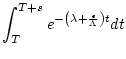 |
(9) | ||
![$\displaystyle \frac{-1}{\left(\lambda + \frac{\epsilon}{\Lambda}\right)}
e^{-\l...
...ight)T}
\left[ e^{-\left(\lambda + \frac{\epsilon}{\Lambda}\right)s} -1 \right]$](img173.png) |
(10) |
whereas the nuclide concentration approximated from trapezoidal integration ![]() is:
is:
| (11) | |||
| (12) |
So the ratio of the approximate to true nuclide concentration is:
![$\displaystyle \frac{N_{trap}}{N_{actual}} = -\frac{s \left(\lambda + \frac{\eps...
...] } { \left[ e^{-\left(\lambda + \frac{\epsilon}{\Lambda}\right)s} -1 \right] }$](img179.png) |
(13) |
Several things are important here. First, this does not depend on ![]() , so it represents the accuracy of the approximation for the entire integration as well as for a single time step. Second, this is always greater than 1, that is, trapezoidal integration always overestimates the nuclide concentration - which eventually results in an underestimate of the exposure age. Although this is accounted for by the fact that reference production rates are calibrated using the same numerical method that is used for the exposure age calculations, it is still important to minimize this inaccuracy. Third, the spallogenic part of the production-depth relationship is the limiting factor in selecting the time step - production by muons can be considered just to have larger
, so it represents the accuracy of the approximation for the entire integration as well as for a single time step. Second, this is always greater than 1, that is, trapezoidal integration always overestimates the nuclide concentration - which eventually results in an underestimate of the exposure age. Although this is accounted for by the fact that reference production rates are calibrated using the same numerical method that is used for the exposure age calculations, it is still important to minimize this inaccuracy. Third, the spallogenic part of the production-depth relationship is the limiting factor in selecting the time step - production by muons can be considered just to have larger ![]() , which is always more accurate for the same
, which is always more accurate for the same ![]() .
.
In practice, for an erosion rate of 10 m ![]() Myr
Myr![]() , that is, 0.001 cm
, that is, 0.001 cm ![]() yr
yr![]() , which would be considered large for accurate exposure dating, the 1000-yr time step used in the calculation yields accuracy at the
, which would be considered large for accurate exposure dating, the 1000-yr time step used in the calculation yields accuracy at the ![]() level, which is clearly adequate for the present purpose. Note that it would not be acceptable for short-half-life radionuclides (e.g.,
level, which is clearly adequate for the present purpose. Note that it would not be acceptable for short-half-life radionuclides (e.g., ![]() C) or high erosion rates.
C) or high erosion rates.
4. Check for saturation.
If the measured nuclide concentration in the sample exceeds the highest calculated value of ![]() for a particular scaling scheme, the sample is taken to be saturated with respect to that scaling scheme. As discussed above, the choice of the maximum length of the forward calculation means that this determination is conservative, that is, samples that are in reality close to saturation may be reported as saturated. Again, if you are interested in rigorous analysis of near-saturated samples, this code is not for you.
for a particular scaling scheme, the sample is taken to be saturated with respect to that scaling scheme. As discussed above, the choice of the maximum length of the forward calculation means that this determination is conservative, that is, samples that are in reality close to saturation may be reported as saturated. Again, if you are interested in rigorous analysis of near-saturated samples, this code is not for you.
5. Error propagation.
We approximate the uncertainty in the exposure age results by solving the simple age equation for an effective scaling factor
![]() for each scaling scheme Xx. This is the scaling factor that, when used in the simple age equation, yields the actual exposure age inferred from the full forward integration described above. Then the effective production rate
for each scaling scheme Xx. This is the scaling factor that, when used in the simple age equation, yields the actual exposure age inferred from the full forward integration described above. Then the effective production rate
![]() . This then allows linear propagation of errors through the simple age equation to arrive at an estimate of the age uncertainty, as follows.
. This then allows linear propagation of errors through the simple age equation to arrive at an estimate of the age uncertainty, as follows.
The internal uncertainty in the exposure age
![]() for scaling scheme Xx is:
for scaling scheme Xx is:
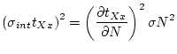 |
(14) |
where ![]() is the standard error in the measured nuclide concentration and:
is the standard error in the measured nuclide concentration and:
![$\displaystyle \frac{\partial t_{Xx}}{\partial N} = \left[ P_{eff,Xx} - N \left( \lambda+\frac{\rho \epsilon}{\Lambda_{sp}} \right) \right]^{-1}$](img195.png) |
(15) |
The external uncertainty in the exposure age
![]() for scaling scheme Xx is:
for scaling scheme Xx is:
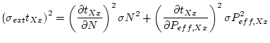 |
(16) |
where
![$\displaystyle \frac{\partial t_{Xx}}{\partial P_{eff,Xx}} = -N \left[ P_{eff,Xx...
...{eff,Xx} \left( \lambda+\frac{\rho \epsilon}{\Lambda_{sp}} \right) \right]^{-1}$](img198.png) |
(17) |
| (18) |
and
![]() is the standard error in the reference production rate for scaling scheme Xx.
is the standard error in the reference production rate for scaling scheme Xx.
![$\displaystyle t_{simple} = \frac{1}{\lambda+\frac{\rho \epsilon}{\Lambda_{sp}}}...
...{P_{sp.St}} \left( \lambda+\frac{\rho \epsilon}{\Lambda_{sp}} \right) \right] }$](img105.png)
![$\displaystyle R_{C} = 14.9 \left( \frac{M}{M_{0}} \right) \left[ cos(\theta) \right]^{4}$](img148.png)