miss = ET_objective(E,cs,target,dFlag)
This is the objective function used by get_al_be_erosion to solve for the erosion rate.
The argument E is the erosion rate.
The argument target is the measured number of atoms to which the predicted value will be compared (atoms ![]() g
g![]() ). Thus, the value of
). Thus, the value of E that yields miss = 0 solves the equation.
The argument cs is a structure with the following fields:
| cs.tv | Time vector (yr) | 1xn double array |
| cs.P_sp_t | Surface production rate due to spallation at times corresponding to those in cs.tv (atoms |
1xn double array |
| cs.z_mu | Vector of depths. This is generally [0 logspace(0,5.3,100)] plus half the sample thickness. That is, we linearize cs.P_mu_z. (g |
1xm double array |
| cs.P_mu_z | Production rates due to muons at depths in cs.z_mu. (atoms |
1xm double array |
| cs.l | Decay constant for nuclide of interest (yr |
double |
| cs.tsf | Thickness scaling factor (nondimensional) | double |
| cs.L | Effective attenuation length for spallogenic production (g |
double |
The argument dflag is a string variable telling the function what to return. If dflag = `no,' the output is just the objective function value, that is, the number of atoms difference between the measured value (target) and that predicted by the supplied erosion rate. If dflag = `yes,' the output is a structure containing diagnostic information, as follows:
| miss.ver | Version number of this function | string |
| miss.Nmu | Nuclide concentration in sample attributable to production by muons at the given erosion rate (atoms |
double |
| miss.Nsp | Nuclide concentration in sample attributable to production by spallation at the given erosion rate (atoms |
double |
| miss.expected_Nsp, miss.PP, miss.A, miss.tsf | Assorted diagnostics. Some are optional - generally depending on whether time-dependent or steady production is being used. | various |
This function calculates the following:
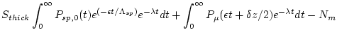 |
(37) |
where ![]() is depth (g
is depth (g ![]() cm
cm![]() ),
), ![]() is the sample thickness (g
is the sample thickness (g ![]() cm
cm![]() ),
), ![]() is the erosion rate (the input argument
is the erosion rate (the input argument E, here in g ![]() cm
cm
![]() yr
yr![]() ),
), ![]() is the measured nuclide concentration (the input argument
is the measured nuclide concentration (the input argument target), ![]() is the surface production rate due to spallation at time
is the surface production rate due to spallation at time ![]() ,
, ![]() is the decay constant of the nuclide of interest,
is the decay constant of the nuclide of interest,
![]() is the effective attenuation length for production by spallation,
is the effective attenuation length for production by spallation, ![]() is the thickness scaling factor (dimensionless) and
is the thickness scaling factor (dimensionless) and
![]() is the thickness-averaged production rate due to muons as a function of depth.
is the thickness-averaged production rate due to muons as a function of depth.
This equation is basically the predicted nuclide concentration in the sample at the given erosion rate, less the measured nuclide concentration. Thus, the correct erosion rate is the value of E for which this function returns zero.
The first term of this equation, that is, the predicted nuclide concentration in the sample attributable to production by spallation, is integrated semi-numerically. We divide it into timesteps to account for surface production rate changes as a function of time, use trapezoidal integration for ![]() (that is, use the average production rate during each time step in that time step) and then integrate each time step analytically. So the nuclide concentration produced in a time step that extends from
(that is, use the average production rate during each time step in that time step) and then integrate each time step analytically. So the nuclide concentration produced in a time step that extends from ![]() to
to ![]() is given by:
is given by:
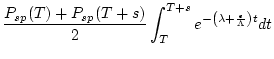 |
(38) | ||
![$\displaystyle -\frac{{P_{sp}(T) + P_{sp}(T+s)}}{2 \left( \lambda + \frac{\epsil...
... T+s \right)}-
e^{-\left( \lambda + \frac{\epsilon}{\Lambda} \right) T}
\right]$](img510.png) |
(39) |
The final time step goes to infinity.
The second term, that is, the predicted nuclide concentration in the sample attributable to production by muons, must be calculated numerically. We do this by transforming the vector of depths at which we have calculated production due to muons to a vector of times (that is, dividing by the erosion rate), then using trapezoidal integration. The upper limit of integration ![]() is
is
![]() . The accuracy of this integration can be evaluated by similar arguments as described in the documentation for
. The accuracy of this integration can be evaluated by similar arguments as described in the documentation for get_al_be_age.m above in section 1.3. The main difference here is that the effective attenuation length for production by muons increases with depth, so the step size can increase with time while still maintaining the same accuracy. Basically, the accuracy is set by the choice of the function argument cs.z_mu. We choose a logarithmic spacing that yields accuracy near or better than ![]() for typical erosion rates.
for typical erosion rates.